Your first Python algorithm with pyDev

This page walks through a complete, very small example: you write a simulation algorithm in a few lines of Python, and G2S runs it. G2S takes care of the simulation path, finds the already-simulated neighbours of each node, handles hard data and threads, and returns the result to your client. Your code only answers one question: given these neighbours, what value should this node get?

The full reference (all parameters, environment selection, batch mode details) is on the pyDev page.

Before you start

You need:

• a G2S server with pyDev built (make pydev, see Build and install), running on the machine where the algorithm file is, because the server reads that file;
• a Python environment with numpy, from the same Python version and build as pyDev (for example a venv created with python3.14t -m venv myenv when pyDev was built against python3.14t);
• the G2S Python client (pip install G2S).

Step 1: write the algorithm

The idea of this toy algorithm: each node gets the inverse-distance weighted mean of its known neighbours, plus a bit of Gaussian noise. Simulated along a random path, this produces a smooth random field that honours the hard data.

Save this as smoothNoise.py:

#!/path/to/myenv/bin/python
import numpy
from statistics import NormalDist

class smoothNoise:
    def __init__(self, TIs, kernel, di, dt, path):
        self.noise = 0.3                          # strength of the random part

    def sample(self, coordinates, values, randUniform, indexInThePath, threadId,
               fullStationary, variableOfInterest, idTI4Sampling):
        v = values[1:, 0]                         # neighbour values (row 0 is the node itself)
        known = ~numpy.isnan(v)
        if not known.any():                       # very first node, nothing known yet
            return 0.0
        d = numpy.linalg.norm(coordinates[1:][known], axis=1)
        w = 1.0 / d**2                            # inverse-distance weights
        mean = numpy.sum(w * v[known]) / numpy.sum(w)
        u = min(max(randUniform, 1e-12), 1 - 1e-12)
        return mean + self.noise * NormalDist().inv_cdf(u)

A few things to note:

• The first line (shebang) selects the Python environment to run the code in. Replace it with the python of your environment. You can leave it out if the Python pyDev was built against already has numpy.
• The class name is the file name, so -pa smoothNoise.py finds it. Another class in the same file can be selected with -pa smoothNoise.py:OtherClass.
• __init__ runs once. It receives the training images, the kernel, the destination image, the data types and the path, in case your algorithm needs them. Here we ignore them.
• sample is called once per node to simulate:
  • coordinates is an int32 (k, ndim) array of offsets from the node (row 0 is the node itself, offset 0);
  • values is a float64 (k, nvar) array with the values at these offsets;
  • randUniform is a random number in [0, 1) for this node, derived from the seed, so runs are reproducible.

  Return the simulated value (or one value per variable).

Step 2: run it from Python

import os
import numpy
import matplotlib.pyplot as plt
from g2s import g2s

di = numpy.full((100, 100), numpy.nan)   # NaN = to simulate
di[20, 20] = 3.0                         # two hard data
di[70, 60] = -3.0

result = g2s('-a', 'pyDev',
             '-pa', os.path.abspath('smoothNoise.py'),
             '-di', di,       # destination image
             '-dt', [0],      # one continuous variable
             '-n', 20,        # 20 known neighbours per node
             '-s', 1,         # seed
             '-j', 4)         # 4 threads

plt.imshow(result['simulation'])
plt.colorbar()
plt.show()

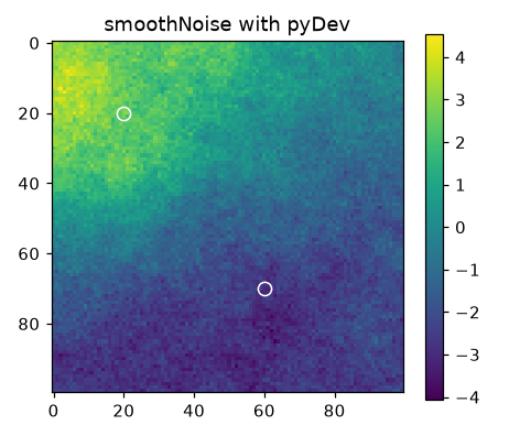
The two hard data (circles) are kept, and the field varies smoothly between them. Run it again with another -s to get another realisation. With the same seed, you get exactly the same image whatever the number of threads.

Instead of an absolute path, you can also copy smoothNoise.py into the server’s PyDevAlgo folder and simply pass '-pa', 'smoothNoise'.

If your code raises an exception, the job stops and the client shows the error. The full Python traceback is in the job log of the server.

Step 3 (optional): predict many nodes at once

Calling Python once per node is fine for quick tests. For machine-learning models, or anything vectorised, it is much faster to predict a whole batch of nodes in one call. Add a sample_batch method to the same class:

    def sample_batch(self, coordinates, values, randUniform, indexInThePath, idTI4Sampling):
        v = values[:, 1:, 0]                                  # (B, K)
        d = numpy.linalg.norm(coordinates[:, 1:], axis=2)     # (B, K)
        w = numpy.where(numpy.isnan(v), 0.0, 1.0 / numpy.maximum(d, 1)**2)
        total = w.sum(axis=1)
        mean = (w * numpy.nan_to_num(v)).sum(axis=1) / numpy.where(total > 0, total, 1)
        u = numpy.clip(randUniform, 1e-12, 1 - 1e-12)
        gauss = numpy.array([NormalDist().inv_cdf(x) for x in u])
        return mean + self.noise * gauss                      # one value per node: (B,)

The arrays gain a first dimension B, the number of nodes in the batch. Nodes with fewer neighbours are padded with NaN values (and offset 0), which is why the weights are set to 0 where the value is NaN.

As soon as the class defines sample_batch, pyDev uses it. Choose the batch size with -bs:

result = g2s('-a', 'pyDev', '-pa', os.path.abspath('smoothNoise.py'),
             '-di', di, '-dt', [0], '-n', 20, '-s', 1, '-bs', 32)
print(result['python_calls'], result['batch_average_size'])

Each node still sees exactly the same neighbours as with sample, so the image is identical to the one of step 2. Only the number of Python calls changes: on this 100 × 100 grid, about 390 calls with batches of 26 nodes on average, instead of 9998 calls. -bs 1 goes back to sample.

Where to go next

• The pyDev reference lists every parameter: kernels (-ki), simulation paths (-sp), training images (-ti), several variables, the index map output, and the optional build() and finalize() methods.
• The PyDevAlgo folder contains complete examples: sequential Gaussian simulation with kriging (sgs, sgsCP, sgsTiCP) and a small neural network trained on a training image (mlpTemplate), a starting point for PyTorch or JAX models.
• Client scripts using them are in example/python/pydev/.